


A Guide to Analysing Rapid Light Curves
Rapid Light Curves can easily be generated with most PAM fluorometers using the program supplied with the instrument you are using. Some fluorometers even provide automated analysis of these curves. However, the default RLC settings may not be ideal for your study, and the curve fitting analysis may also not be suitable for your purposes.
This Guide aims to help you do three things:
- correctly set up your PAM fluorometer,
- choose the best RLC settings for your experimental design or sampling regime, and
- analyse your curves to determine parameter estimates with their estimates of error (we will touch on comparisons between sets of curves).
Detailed discussions of RLC and RLC parameter interpretation are well beyond the scope of this Guide – see White and Critchley (1999) and Ralph and Gademann (2005) for this essential background. Nomenclature is still contested, you could use Van Kooten and Snel (1990) or the more recent Cosgrove and Borowitzka (2011).
After reading this Guide you can expect to have learnt:
- What a RLC is.
- How and why to set up your fluorometer.
- How and why to set up a RLC; and how to run it.
- How to analyse the RLC to determine parameter estimates and their error.
- How to compare RLCs between treatments.
A PDF of this webpage can be found here: How to Analyse a Rapid Light Curve.
First, some background…
What is a Rapid Light Curve?
A typical Rapid Light Curve (or RLC) is derived from a rapid (e.g. 90 second) light treatment applied to a photosynthetic sample (leaf, thallus, culture). During exposure to the treatment light, the photosynthetic capacity (the effective quantum yield of electron transport through photosystem II (PSII), or fPSII) is measured numerous times using the saturation pulse method. A curve treatment may start with a saturating pulse measurement (fPSII) followed by a 10 second interval of exposure to low intensity actinic light and another fPSII measurement, again followed by a 10 second exposure to slightly stronger actinic light and another fPSII measurement. Actinic light is the light provided by the fluorometer that “drives” the photosystem. There may be as few as five steps, typically eight, and possibly more. Values of fPSII generally range from a maximum of around 0.83, indicating 83% of absorbed light energy is directed to PSII, down to 0%.
By plotting fPSII against PAR, we can see how fPSII gradually declines with increases irradiance. However, by calculating photosynthetic rate and plotting this against PAR we generate a light response curve, or PE curve. These curves have been around for many years, and show how photosynthetic rate reaches a maximum at a certain irradiance, among other things.
To estimate photosynthetic rate from each data point, we calculate Electron Transport Rate (ETR) by multiplying fPSII and PAR of the preceding interval, and then multiply this by two constants. If the constants are unknown, simply use “1” to determine relative electron transport rate (rETR). The constants are 1) the absorptance of the sample and 2) the ratio of PSII/(PSII+PSI). Values of calculated rETR or ETR are then plotted against PAR of each interval. A typical curve starts from the origin (0,0) as a line, then levels off (asymptotes) at high irradiances eventually reaching a maximum. Some curves may then decline in ETR with higher PAR, often referred to as photoinhibition. See White and Critchley (1999) for a comprehensive discussion of RLCs, and the later paper by Ralph and Gademan (2005).
An important point to keep in mind is that for most RLCs all the measurements are made on the same section of sample. This means that each data point on the curve is not independent of the other points. Often this is conveniently ignored, and in some situations that is OK. However, it is ultimately up to you to make that call. See White and Critchley (1999) for a discussion on this point.
RLCs indicate the irradiance where maximum ETR is attained, and may also indicate the onset of apparent photoinhibition at greater irradiances.
What other measurements should I make when I run a Rapid Light Curve?
- Photosynthetically Active Radiation (PAR): electron transport rate can only be calculated with a value for incident light. In units mmols quanta m-2 s-1.
- Absorptance: this is often assumed to be 0.84, however this value can vary significantly within and between individuals and species. This is also used to calculate electron transport rate
- PSII/(PSI+PSII): the proportion of energy directed to photosystem II, often assumed to be 0.5 but can deviate from this value
These values (PAR, Absorptance and PSII(PSI+PSII)) are used with fPSII to calculate Electron Transport Rate (ETR) according to Genty’s equation (or relative ETR (rETR) if Absorptance and/or PSII(PSI+PSII) are not known):

What data can be derived from a Rapid Light Curve?
- ΦPSII immediately commencing the RLC
- ΦPSII at the measured ambient irradiance, interpolated from the curve
- ETR associated with each saturating pulse measurement made during the curve. In units mmol e m-2 s-1.
- ETRmax: the maximum ETR attained. In units mmol electrons m-2 s-1.
- α or alpha; the initial slope of the curve. In units electrons/quanta (only use these units when actual ETR is determined, not rETR).
- Ek: the minimum saturation irradiance, where maximum ETR would be reached if there was no inflection in the curve (i.e. extrapolate the initial linear part of the curve to intersect with maximum ETR (or rETR). In units mmol quanta m-2 s-1.
- β or beta, a little used parameter that characterises the downturn of the curve after reaching ETRmax.
Now, to set up your PAM for optimal results…
Setting up your PAM fluorometer
Clear a space, grab your PAM fluorometer and a test sample, or random leaf if you are just getting used to the procedure.
- Prepare the test sample for setup measurements. Preferably choose a sample that has not been subjected to strong light.
- Saturating Pulse (SP) duration: Select your duration of the saturation pulse (often known as the saturation width): g. 800 ms is often used when examining a leaf.
- SP intensity: select the intensity of the saturating pulse. Often the default setting is adequate. Ideally, select an intensity that will provide a saturating curve rather than a stepwise function between fluorescence values of F and Fm. If the latter, reduce the intensity until the a curve is generated.
- AUTOGAIN: If your PAM fluorometer has the function, select AutoGain or its equivalent. This will set the gain of the fluorometer to a suitable level. If your fluorometer requires you to manually set the gain, select a gain value where the F value of an unstressed sample (i.e. collected early in the morning) is about one eighth (0.125) the highest acceptable Fm value. For example, if the maximum value on the PAM is 4000 units, then the gain should be set so the F value of an unstressed sample is less than 400 units. This will ensure that highest expected value of Fm does not exceed the instrument maximum.
- AUTOZERO: Now remove the sample from the measuring area of the PAM fluorometer, ensure nothing else that might fluoresce will be seen by the fluorometer, and select AutoZero. F should now read around zero. If your fluorometer requires you to manually set zero, take an average of the F value and subtract this value from all subsequent values
- Test Measurement: take a measurement on a fresh part of the same leaf or sample. If the sample is an unstressed green leaf subjected to low light for at least an hour one might expect a fPSII value between 0.7 to 0.83. Much less than this and you may want to repeat the setup procedure again on a new sample, to be sure.
Constructing and running a RLC
Now that you have set up your PAM fluorometer for making useful ΦPSII and Fv/Fm measurements, let’s focus on the RLC settings.
- Actinic intervals: You’ll need to set the intensity of the actinic light during each interval. Different fluorometers provide different options for setting the actinic light intensity. The ideal settings will generate several data points when light intensity is low and the curve is a straight line, and several data points at high light intensity to capture the saturating nature of the curve. If you are more interested what is happening under low light conditions, then you will obtain a better estimate of a with more low-light data points.
- Actinic interval duration: The duration of each interval or step can generally be altered from 10 seconds(typical) to 30 seconds or more. At some duration of interval Rapid Light Curves are no longer rapid. The functional definition of “rapid” is largely based on the premise that for a curve to be rapid, fundamental changes in the photochemistry of the sample have not yet had sufficient time to occur. This is incorrect when it comes to changes in energy-dependent non-photochemical quenching (qE), as processes described by this parameter are activated and de-activated within seconds. physiological processes that take longer to be induced can be assumed to be largely unchanged during the RLC.
Running the RLC
This is the easy part. Most of the hard work is done before and after generating the curve!
- Place the sample of interest in the position where it is to be measured (either over the window of the PAM fluorometer, in the sample holder clip or in front of the fibre optic leading from the fluorometer). Ensure the sample will not move during the RLC procedure (very important).
- Exclude ambient light from the sample. Complete darkness is not necessary, but less light than that provided during the first actinic interval is best.
- Initiate the curve, ensuring darkness (apart from the fluorometer light) is maintained. It is essential the sample does not move for the entire duration of the treatment. If it moves, fluorescence intensity is likely to change as you will be looking at a new section of sample, and subsequent measurements cannot be related to the first measurements.
Running a Recovery Curve after the RLC
With increasing light intensity, fPSII declines. When the “light pressure” is removed at the end of the RLC treatment, fPSII “bounces back”, gradually increasing until, if still in darkness, Fv/Fm will be reached. The kinetics of this recovery can be examined by analysis of a so-called Recovery Curve. Recovery of a process from a high light treatment is best modelled with an exponential function. Recovery typically comprises two (or sometimes three) processes, each with different halftimes and this can be modelled with a double exponential model. The majority of recovery occurs rapidly (within minutes), and the remainder can take a long time to fully recover (hours). So, the ideal measurement regime to capture the recovery of a photosynthetic sample to a high light treatment takes the form of many measurements taken during the initial recovery phase with progressively less frequent measurements taken at longer and longer intervals.
How to extract data from a RLC
Preparation of the RLC graph
Let’s assume you measured the actinic PAR at each interval of a light curve, correctly set up the gain and zero settings of the PAM fluorometer, and ensured the sample remained fixed during the measurements with minimal ambient light reaching the sample. The PAM fluorometer provides you with fPSII values measured at the end of each interval.
- Assemble the PAR values for each interval in Column A (starting with zero), and in Column C add the corresponding fPSII The first fPSII value corresponds with the zero PAR value. This value is actually not used in most RLCs, as electron transport is assumed to be zero in the dark.
- Now in Column B, multiply the fPSII values with values for absorptance and PSII/(PSII+PSI). If you do not have these values, you will only be able to present values of relative ETR (rETR).
- Create a line graph of ETR (y-axis) vs PAR (x-axis). The initial part of the line extending from the origin should be straight, with the latter part forming a curve which approaches or reaches a maximum (the asymptote). You may find the curve then curves downwards again with even higher irradiances.
Analysis of the RLC – models
The aim here is to extract values of the parameters ETRmax, Ek and a and potentially estimates of error associated with these values from your data. The data we use is simply the two columns, PAR and ETR.
There are a multitude of models that have been used to describe RLCs and more generally PE curves. Each model, or equation, assumes a particular relation between the parameters. Some models introduce new parameters that do not have a direct biological meaning and should only be used if that model addresses a specific problem. Ideally, a model should have functions that directly describe known processes. For example, single-or multi-compartment exponential models are best used to describe recovery curves, as exponential decay best describes the relaxation of physiological processes that were induced by the light treatment and causes a depression in fPSII.
PE curve modellers tend to have their own favourite models they use to describe RLCs. As many of my curves were either simple asymptotes, or were both asymptotic with a downturn at higher irradiances, I selected a model that enabled me to analyse both types of curves. This model comprises two terms: one two-parameter term for the asymptote, and a second term (with a third parameter) which could be added if the curve also experienced a downturn. The second term could be excluded if there was no downturn. This approach is important as one can only compare parameters derived from models with the same fundamental basis, parameters derived from fundamentally different models are incompatible and should not be compared directly.
The model describing RLCs that have no downturn at high irradiances (i.e. a simple asymptote) is:
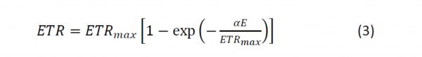
This model is modified with an additional term to account for a downturn in ETR:

Where ETRs is a scaling parameter defining the maximum potential photosynthetic rate, and b represents the slope of the downturn part of the curve, often referred to as photoinhibition.
ETRmax is then calculated from the following:
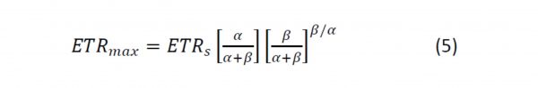
See Frenette et al. (1993) for a detailed discussion.
Non-linear regression assumes a few attributes of your data; the following statements should be true (or mostly true):
- PAR values (x axis values) are accurate, while ETR values (y axis values containing fII) are less accurate and contain the variability we are interested in,
- The variability of possible ETR values associated with a particular PAR value would be distributed normally and follow a bell curve – or put another way, there is no reason to expect ETR values associated with a particular PAR value to be overrepresented by higher or lower values than the mean value.
- The standard deviation of each residual at each data point is similar in magnitude across the entire curve, or if weighted then the pattern is predictable,
- Each ETR value is independent of any other ETR value that might be measured at that same PAR value.
See Motulsky and Christopoulos (2013) for an accessible and more detailed discussion of assumptions inherent in non-linear regression methods.
Analysis of the RLC – using a spreadsheet
Once you have selected the model you want to use (simple asymptotic model, or model with downturn), what next? You can use a statistics package – look for “non-linear least squares regression” as this is the technique used. Most applications employ the Levenberg-Marquardt algorithm. Type in your model and copy and paste your data set into the program. You may be asked to enter “seed” values, which are your best estimate values of ETRmax, a and Ik (ETRmax and Ik are easily obtained by eye from a graph of the RLC, a is calculated as ETRmax/Ek). Some applications may only offer a standard set of models and not allow you to create your own.
You may want to avoid the expense of purchasing a statistics package. A spreadsheet with a Solver function can easily determine the parameter estimates (Brown 2001). However a macro will be needed if you want to determine the estimates of error associated with each parameter. Better still learn to use the open source statistics software “R”, and search for “non-linear least squares regression” for guidance. By learning to use R you can then address most statistical problems with mathematical rigour.
Rather than explain the details in words, I have created two spreadsheets you can use. These can be found at https://aquation.com.au/tools/calculators/. One spreadsheet simply calculates the parameter estimates for both a two-parameter curve and a three-parameter curve using the Solver function in Microsoft Excel. Instructions are in the spreadsheet. I suggest copying one of the worksheets to a new sheet within the workbook and experimenting with different models to see how it works.
Determining the error associated with each parameter estimate is more difficult and requires a multistep process that is apparently best done using a macro. Rather than reinvent the wheel, I’ve provided an Excel add-in courtesy of Leonardo Volpi and the Foxes Team, Italy. You can find more information relating to this and other complex analysis in Excel at Professor Robert de Levie’s site http://www.bowdoin.edu/~rdelevie/excellaneous/.
Running the Solver-based model (parameter estimates only)
Enter your data, and suitable estimates for ETRmax and alpha. Select Solver and run it, minimising the Sum of Squares, and optimising the parameters ETR and alpha. Note the slope of the curve must always be positive, this can be inserted in Solver as a condition. Observe the two lines in your figure, the modelled data should converge with the observed data. If the modelled data suddenly produce a curve that does not approximate the observations at all, you will need to select better estimates of the model parameters.
If you have set it up correctly, the parameter values should fluctuate during the iterative curve fitting procedure and settle down quickly so that just the last decimal places of the estimates continue to vary for a few iterations before the program stops. The R2 value represents the proportion of data that the model describes, so an R2 of 1.0 would mean that 100% of the data is explained by the model.
Running the Macro-based model (includes error estimates for parameters)
Enter your data, and suitable estimates for ETRmax and alpha. Follow the instructions on the spreadsheet to activate and run the Optimiz macro (Using Addins for Excel). Estimates of error for your parameters should be included as Standard Deviation, and 95% Confidence Interval. The R2 value represents the proportion of data that the model describes, so an R2 of 1.0 would mean that 100% of the data is explained by the model. Estimates of error and R2 described here should be considered as indicative. The calculation of error estimates for the parameters, and an R2 value for the curve itself is a complex topic with subtleties better described elsewhere.
How to compare RLCs between treatments
Pooling and comparing curve data
One may obtain several RLCs on separate replicate plants or leaves in a treatment or plot and wish to pool or compare these treatments. There are multiple approaches available. You need to be the final judge of what is best used considering your data and experimental or survey design. See Peek et al. (2002) for a useful discussion.
Replicates: pooling data of all curves is the simplest method. If each of three curves has eight data pairs, then the pooled curve will have 24 -2 = 22 data pairs (the origin (0,0) need not be repeated). A single analysis on this curve will provide single estimates for ETRmax and alpha, and an estimate of Ek can be determined from these. Error associated with the parameter estimates will capture the variability or scatter of data points of all the curves. An alternative approach often used is to analyse each curve individually, derive the parameter estimates and calculate the mean and error of this set of estimates. This approach is not recommended as it does not describe the variability associated with each individual curve. This is because only the parameter estimate is carried over when combining data (by averaging) from the multiple curves.
Comparisons: Often investigators will perform RLCs on several samples relating to a treatment, and then repeat the process for samples from another treatment, with the intention of performing a simple T test (if two treatments) or analysis of variance (or more than two treatments) to determine whether the curves indicate a significant difference between treatments. However, as discussed above, analysis of just the parameter estimates from each curve ignores the extent of variability within each curve (i.e. the amount of scatter), and is therefore not an ideal approach.
Analysing Recovery Curves
Recovery curves are obtained from repeated saturating pulse measurements after a light treatment (e.g. RLC) but while ambient light is still excluded. Recovery from a high light event is generally seen as a rapid rise in yield that quickly (within minutes) slowing to a more gradual increase in yield, eventually reaching a maximum after hours to days, depending on the severity of the light treatment. Both rapidly- and slowly-recovering processes can be described with exponential terms, usually in the form of a double exponential model.
We have already discussed the use of non-linear models to analyse RLCs. The application of the double exponential model to recovery curves is very similar. In this instance, rather than address changes in ETR (which depend on there being a positive value of PAR), we can address changes in ΦII, F or Fm.
References.
BROWN, A.M. (2001). A step-by-step guide to non-linear regression analysis of experimental data using a Microsoft Excel spreadsheet. Comp. Methods Prog. Biomed. 65, 191-200
FRENETTE, J.-J., DEMERS, S., LEGENDRE, L. & DODSON, J. (1993). Lack of agreement among models for estimating the photosynthetic parameters. Limnol. Oceanogr., 38, 679-687.
GENTY, B., BRIANTIAS, J. M. & BAKER, N. R. (1989). The relationship between the quantum yield of photosynthetic electron transport and quenching of chlorophyll fluorescence. Biochim. Biophys. Acta 990, 87-92.
MOTULSKY, H. & CHRISTOPOULOS, A. (2003). Fitting models to biological data using linear and non-linear regression: a practical guide to curve fitting. Oxford University Press, Oxford.
PEEK, M.S., RUSSEK-COHEN, E. WAIT, D.A., & FORSETH, I.N. (2002). Physiological response curve analysis using nonlinear mixed models. Oecologia 132, 175–180
RALPH, P.J. & GADEMANN, R. (2005). Rapid light curves: a powerful tool to assess photosynthetic capacity. Aquat. Bot., 82: 222–237.
WHITE, A.J., & CRITCHLEY, C. (1999). Rapid light curves: a new fluorescence method to assess the state of the photosynthetic apparatus. Photosynth. Res., 59, 63–72.
VAN KOOTEN, O & SNELL, JFH. (1990). The use of chlorophyll fluorescence nomenclature in plant stress physiology. Photosynth. Res 25, 147–150